Introduction
A geophone is a ground motion sensor that converts mechanical vibrations into electrical signals. It is widely used in seismic vibration detection, earthquake monitoring, structural health monitoring, and military applications.
Working Principle
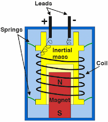
Geophones operate on the basis of electro-magnetic induction. The main parts include:
Inertial Mass (Proof Mass): A suspended magnet or coil that moves relative to the geophone housing due to ground movement.
Spring System: Keeps the mass in neutral position and allows it to oscillate when subjected to vibrations.
Coil-Magnet Assembly:
If the coil is fixed and the magnet moves, a voltage is induced (Faraday’s law).
Conversely, if the magnet is fixed and the coil moves, the same principle applies.
The induced voltage ($V$) is proportional to the velocity of the mass relative to the housing:
$$V = -G \cdot v$$
where:
$G =$ Transduction coefficient (V$\cdot$s/m), defined as $G = N \cdot B \cdot L$
$N =$ Number of coil turns
$B =$ Magnetic field strength (Tesla)
$L =$ Length of the coil wire in the field (meters)
$v =$ Relative velocity (m/s)
Frequency Response & Damping
Geophones are velocity sensors, meaning they measure ground velocity rather than displacement or acceleration. The response depends on:
Natural Frequency ($f_n$): Determined by the spring-mass system.
$$f_n = \frac{1}{2\pi}\sqrt{\frac{k}{m}}$$
where $k =$ spring stiffness, $m =$ inertial mass.
Damping Ratio ($\zeta$): Controls the rate at which oscillations decay.
Critical damping ($\zeta = 0.707$) is often used for optimal transient response.
The total damping includes both mechanical damping and electrical damping:
$$\zeta = \frac{1}{2}\left[\frac{c + G^2/R_{tot}}{\sqrt{km}}\right]$$
where $c$ is the mechanical damping coefficient and $R_{tot}$ is the total resistance in the circuit.
Transfer Functions
The geophone can be represented by different transfer functions depending on the input of interest:
Displacement to Voltage Transfer Function
The frequency response relating output voltage to input displacement is:
$$\frac{V(s)}{X(s)} = \frac{Gs}{1 - \left(\frac{\omega}{\omega_n}\right)^2 + 2j\zeta\left(\frac{\omega}{\omega_n}\right)}$$
where:
$V(s) =$ Output voltage
$X(s) =$ Input displacement
$G =$ Transduction coefficient (V$\cdot$s/m)
$\omega_n =$ Natural angular frequency ($2\pi f_n$)
$\zeta =$ Damping ratio
Acceleration to Voltage Transfer Function
Since acceleration $A(s) = s^2X(s)$ in the Laplace domain, the transfer function from acceleration to voltage is:
$$H(s) = \frac{V(s)}{A(s)} = \frac{Gs}{s^2 + 2\zeta\omega_n s + \omega_n^2}$$
This form is particularly useful for understanding the geophone’s high-pass filtering behavior.
Key Specifications
| Parameter | Description |
|---|---|
| Sensitivity | Typically 20–80 V/(m/s) (higher = better for weak signals) |
| Natural Frequency ($f_n$) | 4.5 Hz (low-frequency) to 100 Hz (high-frequency) |
| Damping Ratio ($\zeta$) | 0.6–0.7 (optimized for flat response near $f_n$) |
| Coil Resistance | 100–10,000 $\Omega$ (affects signal conditioning) |
| Operating Range | 0.5 to 5 cm/s (depends on design) |
Advantages & Limitations
Advantages:
Passive (no external power needed)
High sensitivity at resonant frequency
Rugged and reliable
Limitations:
Limited low-frequency response (unless using a low-$f_n$ geophone)
Susceptible to tilt and temperature variations
Requires signal conditioning for digitization
Comparison with Accelerometers
| Feature | Geophone | Accelerometer |
|---|---|---|
| Output: | Velocity | Acceleration |
| Frequency Range: | Best near $f_n$ | Wider (DC to kHz) |
| Power Requirement: | Passive | Active (needs power) |
| Low-Frequency Performance: | Poor (unless low $f_n$) | Excellent |
Mathematical Model for Geophone Sensing
Basic Model
A geophone behaves as a spring-mass-damper system with an additional electrical damping effect due to the coil resistance and external resistor. The governing equation is:
$$m\ddot{x} + c\dot{x} + kx = F_{ext}$$
where:
$m =$ moving mass (kg)
$c =$ mechanical damping coefficient (N$\cdot$s/m)
$k =$ spring constant (N/m)
$x =$ displacement (m)
$F_{ext} =$ external force (N)
Electrical Domain
Since the geophone outputs a voltage proportional to velocity $v = \dot{x}$, we transform this equation into the electrical domain.
Using Faraday’s Law, the induced voltage in the coil is:
$$V_o = G\dot{x}$$
The geophone circuit consists of the coil resistance $R_c$ and an external damping resistor $R_s$, forming the total impedance:
$$R_{tot} = R_c + R_s$$
which introduces an electrical damping force:
$$F_e = \frac{G^2}{R_{tot}}\dot{x}$$
Complete Equation of Motion
Thus, the equation of motion for the geophone in sensing mode is:
$$m\ddot{x} + \left(c + \frac{G^2}{R_{tot}}\right)\dot{x} + kx = 0$$
Taking the Laplace Transform (assuming zero initial conditions):
$$ms^2X(s) + \left(c + \frac{G^2}{R_{tot}}\right)sX(s) + kX(s) = 0$$
Rewriting in standard second-order system form:
$$s^2X(s) + 2\zeta\omega_n sX(s) + \omega_n^2X(s) = 0$$
where:
Natural Frequency: $$\omega_n = \sqrt{\frac{k}{m}}$$
Damping Ratio: $$\zeta = \frac{1}{2}\left[\frac{c + G^2/R_{tot}}{\sqrt{km}}\right]$$
Transfer Function
Finally, the transfer function from acceleration to voltage output is:
$$H(s) = \frac{V_o(s)}{A(s)} = \frac{Gs}{s^2 + 2\zeta\omega_n s + \omega_n^2}$$
where $A(s)$ represents the input acceleration in the Laplace domain: $A(s) = s^2X(s)$
This transfer function describes the relationship between acceleration input and voltage output. The geophone acts as a high-pass filter, meaning:
The output voltage $V_o(t)$ is proportional to the velocity $\dot{x}(t)$ of the moving mass.
The system is sensitive to motion at frequencies primarily above its natural frequency.
The transfer function helps interpret geophone data for vibration and seismic sensing.
MATLAB Implementation
Below is the MATLAB script to model the geophone system:
% Parameters
m = 0.02; % Moving mass (kg)
k = 1000; % Spring constant (N/m)
c = 0.5; % Mechanical damping (Ns/m)
G = 0.1; % Transduction coefficient (Vs/m)
Rc = 100; % Coil resistance (Ohm)
Rs = 500; % External resistor (Ohm)
Rtot = Rc + Rs; % Total resistance
% Derived parameters
wn = sqrt(k/m); % Natural frequency (rad/s)
zeta = (c + (G^2 / Rtot)) / (2 * sqrt(k*m)); % Damping ratio
% Transfer function
H(s) = Gs / (s^2 + 2*zeta*wn*s + wn^2)
num = [G 0]; % Numerator (Gs)
den = [1 2*zeta*wn wn^2]; % Denominator (s^2 + 2*zeta*wn*s + wn^2)
sys = tf(num, den);
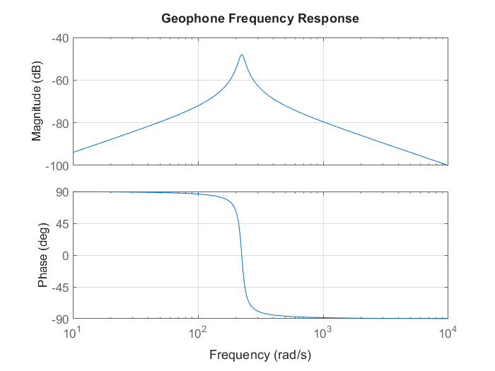
% Plot Frequency Response
bode(sys);
grid on;
title('Geophone Frequency Response');
This MATLAB code defines the geophone sensing transfer function and
plots the frequency response to analyze its behavior.
Conclusion
Geophones are useful for velocity-based vibration sensing in geophysical and industrial applications. Their design focuses on electromagnetic induction, resonant frequency, and damping to ensure accurate detection of vibrations. If you want to meeasure ultralow frequencies alternatives such as broadband seismometers or MEMS accelerometers may be used over geophones.
References
- Prof. Henri P Gavin(W.H. Gardner Jr. Chair of Civil and Environmental Engineering, Professor in the Department of CEE, Duke University)
- KTM GeoLab